Chapter 06 "복잡한 데이터 표현하기"
Chapter 06-2의 주제는 '맷플롯립의 고급 기능 배우기' 이다.
전체적으로 배울 내용은 다음과 같다
- 맥플롯립의 고급 기능
- 하나의 피겨에 다양한 그래프
06-2 맥플롯립의 고급 기능 배우기
실습 준비
# 코랩에서 한글다운
import sys
if 'google.colab' in sys.modules:
  !echo 'debconf debconf/frontend select Noninterative'| \
  debconf-set-selections
  # 나눔 폰트 설치
  !sudo apt-get -qq -y install fonts-nanum
  import matplotlib.font_manager as fm
  fm._rebuild()

# 다시 실행
import matplotlib.pyplot as plt
import gdown
import pandas as pd
# 나눔바른고딕 폰트로 설정
plt.rc('font', family='NanumBarunGothic')
# 그래프 DPI 기본값 변경
plt.rcParams['figure.dpi'] = 100
# ns_book7 다운
gdown.download('https://bit.ly/3pK7iuu','ns_book7.csv', quiet = False)
# pandas dataframe
ns_book7 = pd.read_csv('ns_book7.csv', low_memory = False)
ns_book7.head()
하나의 피겨에 여러 개의 선 그래프 그리기
# 상위 30개 출판사
top30_pubs = ns_book7['출판사'].value_counts()[:30]
top30_pubs_idx = ns_book7['출판사'].isin(top30_pubs.index)

# 상위 30개에 해당하는 '출판사', '발행년도', '대출건수' 만 추출
ns_book9 = ns_book7[top30_pubs_idx][['출판사', '발행년도', '대출건수']]

# '출판사', '발행년도' 기준으로 행을 모은 후 '대출건수'열의 합
ns_book9 = ns_book9.groupby(by = ['출판사', '발행년도']).sum()

# 인덱스 초기화 후 '황금가지' 확인
ns_book9 = ns_book9.reset_index()
ns_book9[ns_book9['출판사'] == '황금가지'].head()
선 그래프 2개 그리기
# 출판사별 데이터프레임
line1 = ns_book9[ns_book9['출판사'] == '황금가지']
line2 = ns_book9[ns_book9['출판사'] == '비룡소']

# line1과 line2 로 plot함수 두 번 호출
fig, ax = plt.subplots(figsize = (8, 6))
ax.plot(line1['발행년도'], line1['대출건수'])
ax.plot(line2['발행년도'], line2['대출건수'])
ax.set_title('연도별 대출건수')
fig.show()
# 범례 추가
fig, ax = plt.subplots(figsize = (8, 6))
ax.plot(line1['발행년도'], line1['대출건수'], label = '황금가지') # 레이블 추가
ax.plot(line2['발행년도'], line2['대출건수'], label = '비룡소')
ax.set_title('연도별 대출건수')
ax.legend() # 범례 추가
fig.show()
선 그래프 5개 그리기
# 상위 5개 출판사
fig, ax = plt.subplots(figsize = (8, 6))
for pub in top30_pubs.index[:5]:
  line = ns_book9[ns_book9['출판사'] == pub]
  ax.plot(line['발행년도'], line['대출건수'], label = pub)
ax.set_title('연도별 대출건수')
ax.legend()
ax.set_xlim(1985, 2025) # x축 범위 설정
fig.show()
스택 영역 그래프
- 스택 영역 그래프: 하나의 선 그래프 위에 다른 선 그래프를 차례대로 쌓는 것
- stackplot()로 구현
- pivot_table() 메서드로 각 '발행년도' 열의 값을 열로 바꾸기
- '발행년도' 열을 리스트 형태로 바꾸기
- stackplot() 메서드로 스택 영역 그래프 그리기
# 1 번 : pivot_table() 메서드로 각 '발행년도' 열의 값을 열로 바꾸기
ns_book10 = ns_book9.pivot_table(index = '출판사', columns = '발행년도')
ns_book10.head()
ns_book10.columns[:10]
# 결과
# MultiIndex([('대출건수', 1947),
#           ('대출건수', 1974),
#           ('대출건수', 1975),
#           ('대출건수', 1976),
#           ('대출건수', 1977),
#           ('대출건수', 1978),
#           ('대출건수', 1979),
#           ('대출건수', 1980),
#           ('대출건수', 1981),
#           ('대출건수', 1982)],
#          names=[None, '발행년도'])
# 2 번 : '발행년도' 열을 리스트 형태로 바꾸기
top10_pubs = top30_pubs.index[:10]
year_cols = ns_book10.columns.get_level_values(1)# 3 번 : stackplot() 메서드로 스택 영역 그래프 그리기
fig, ax = plt.subplots(figsize = (8, 6))
ax.stackplot(year_cols, ns_book10.loc[top10_pubs].fillna(0),
labels = top10_pubs)
ax.set_title('연도별 대출건수')
ax.legend(loc = 'upper left') # 범례 위치
ax.set_xlim(1985, 2025) # x축 범위 설정
fig.show()
하나의 피겨에 여러 개의 막대 그래프 그리기
fig, ax = plt.subplots(figsize = (8, 6))
ax.bar(line1['발행년도'], line1['대출건수'], label = '황금가지') # 레이블 추가
ax.bar(line2['발행년도'], line2['대출건수'], label = '비룡소')
ax.set_title('연도별 대출건수')
ax.legend() # 범례 추가
fig.show()
막대가 덮어쓰였다.
기본 너비인 0.8이 아닌 0.4로 두 막대를 그린 후 x축에서 막대 하나 너비인 0.4의 절반씩 떨어뜨린다.
# 기본 너비인 0.8이 아닌 0.4로 두 막대를 그린 후 x축에서 막대 하나 너비인 0.4의 절반씩 떨어뜨리기
fig, ax = plt.subplots(figsize = (8, 6))
ax.bar(line1['발행년도']-0.2, line1['대출건수'], width = 0.4, label = '황금가지') # 레이블 추가
ax.bar(line2['발행년도']+0.2, line2['대출건수'], width = 0.4, label = '비룡소')
ax.set_title('연도별 대출건수')
ax.legend() # 범례 추가
fig.show()
스택 막대 그래프
- bar() 함수의 bottom 매개변수
height1 = [5, 4, 7, 9, 8]
height2 = [3, 2, 4, 1, 2]

plt.bar(range(5), height1, width = 0.5)
plt.bar(range(5), height2, bottom = height1, width = 0.5)
plt.show()
# 그리기 전에 막대의 길이를 누적
height3 = [a + b for a, b in zip(height1, height2)]

plt.bar(range(5), height1, width = 0.5)
plt.bar(range(5), height2, width = 0.5)
plt.show()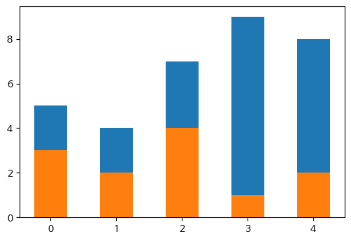
데이터값 누적하여 그리기
- 판다스 데이터프레임의 cumsum() 메서드
# 상위 5개 출판사의 2013~2020 대출건수
ns_book10.loc[top10_pubs[:5], ('대출건수',2013):('대출건수', 2020)]
# 상위 5개 출판사의 2013~2020 대출건수
ns_book10.loc[top10_pubs[:5], ('대출건수',2013):('대출건수', 2020)].cumsum()
# 변수에 저장
ns_book12 = ns_book10.loc[top10_pubs].cumsum()

# plot
fig, ax = plt.subplots(figsize = (8, 6))

# 가장 큰 막대부터 그려야 하므로 누적 합계가 가장 큰 마지막 출판사부터 그림
for i in reversed(range(len(ns_book12))):
  bar = ns_book12.iloc[i]
  label = ns_book12.index[i]
  ax.bar(year_cols, bar, label=label)
ax.set_title('연도별 대출건수')
ax.legend(loc='upper left')
ax.set_xlim(1985, 2025)
fig.show()
원 그래프 그리기
pie chart는 3시부터 반시계방향으로 그려진다.
# 데이터 변수
data = top30_pubs[:10]
labels = top30_pubs.index[:10]

# pie chart
fig, ax = plt.subplots(figsize = (8,6))
ax.pie(data, labels = labels)
ax.set_title('출판사 도서 비율')
fig.show()
원 그래프의 단점
- 어떤 데이터가 더 큰지 한눈에 구별이 어렵다
- startangle 매개변수 = 90 으로 설정하면 12시부터 원그래프를 그림
plt.pie([10, 9], labels = ['A제품', 'B제품'], startangle = 90)
plt.title('제품의 매출 비율')
plt.show()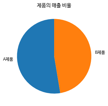
비율 표시하고 부채꼴 강조하기
- pie() 메서드
- autopct 매개변수: % 연산자에 적용할 포맷팅 문자열 전달
- %d이면 각 부채골의 비율이 정수로 표현
- explode 매개변수: 떨어뜨리길 원하는 조각의 간격을 반지름의 비율로 지정
- '문학동네'만 떼어내려면 첫 번째 항복이 0.1이고 나머지는 모두 0인 리스트를 넣어야 함. 리스트는 data 배열의 길이와 같아야 함.
# 비율 표시하고 부채꼴 강조하기
fig, ax = plt.subplots(figsize = (8,6))
ax.pie(data, labels = labels, startangle = 90,
       autopct = '%.1f%%', explode = [0.1]+[0]*9)
ax.set_title('출판사 도서 비율')
fig.show()
여러 종류의 그래프가 있는 서브플롯 그리기
- 지금까지 그렸던 그래프를 하나의 피겨에 그려보기
fig, axes = plt.subplots(2, 2, figsize = (20,16))

# 산점도
ns_book8 = ns_book7[top30_pubs_idx].sample(1000, random_state=42)
sc = axes[0, 0].scatter(ns_book8['발행년도'], ns_book8['출판사'],
           linewidths=0.5, edgecolors = 'k',alpha = 0.3,
           s = ns_book8['대출건수']**1.3, c = ns_book8['대출건수'], cmap='jet')
axes[0, 0].set_title('출판사별 발행 도서')
fig.colorbar(sc, ax = axes[0, 0])
# 스택 영역 그래프
axes[0, 1].stackplot(year_cols, ns_book10.loc[top10_pubs].fillna(0),
             labels = top10_pubs)
axes[0, 1].set_title('연도별 대출건수')
axes[0, 1].legend(loc = 'upper left')
axes[0, 1].set_xlim(1985, 2025)

# 스택 막대 그래프
for i in reversed(range(len(ns_book12))):
  bar = ns_book12.iloc[i]
  label = ns_book12.index[i]
  axes[1, 0].bar(year_cols, bar, label=label)
axes[1, 0].set_title('연도별 대출건수')
axes[1, 0].legend(loc='upper left')
axes[1, 0].set_xlim(1985, 2025)

# 원 그래프
axes[1, 1].pie(data, labels = labels, startangle = 90,
       autopct = '%.1f%%', explode = [0.1]+[0]*9)
axes[1, 1].set_title('출판사 도서 비율')

fig.savefig('all_in_one.png')
fig.show()
기본미션

선택미션
- pivot_table() 메서드로 각 '발행년도' 열의 값을 열로 바꾸기
- '발행년도' 열을 리스트 형태로 바꾸기
- stackplot() 메서드로 스택 영역 그래프 그리기
나머지 코드 실행과 결과는 위에 있음('스택 영역 그래프')
실습코드
https://colab.research.google.com/drive/1kPF2aVPQm3IzngEKtSRcIh2SVsmzp5MR?usp=sharing
혼공분석_6주차-2.ipynb
Colaboratory notebook
colab.research.google.com
4주차부터 미루다가....그래도 유종의 미를 거두기 위해 몰아서 했다.
힘들지만 그래도 시각화 공부는 필요하고 중요하다고 생각했기 때문에 열심히 했다.
그래도 끝을 내서 다행이다!
또 원래 코랩으로 하고싶던 고양이모드가 작동이 돼서 실제로 고양이가 보였다
덕분에 지루하진 않았다.

'Data Analysis > 혼공학습단9기' 카테고리의 다른 글
| 회고록 (0) | 2023.02.26 |
|---|---|
| 혼자 공부하는 데이터 분석 with 파이썬: 6주차(Chapter 06-1) (0) | 2023.02.19 |
| 혼자 공부하는 데이터 분석 with 파이썬: 5주차(Chapter 05-2) (0) | 2023.02.19 |
| 혼자 공부하는 데이터 분석 with 파이썬: 5주차(Chapter 05-1) (0) | 2023.02.19 |
| 혼자 공부하는 데이터 분석 with 파이썬: 4주차(Chapter 04-2) (0) | 2023.02.19 |


